Everything in PDV
Protein Design Viz is a single-file, offline molecular visualization studio that runs entirely in your browser. This guide walks through every feature, from loading structures to publication-ready renders.
1Overview
PDV opens straight in a browser tab, nothing to install, no account, no upload. Your structures never leave your machine.
PDV is built as an extensive modification of 3Dmol.js, the open-source WebGL molecular rendering library, which powers the underlying 3D view. If you use PDV in published work, please also cite 3Dmol.js: Nicholas Rego & David Koes, “3Dmol.js: molecular visualization with WebGL,” Bioinformatics 31(8):1322–1324 (2015). 3Dmol.js is distributed under the BSD-3-Clause license.
Single file, offline
The whole studio is one self-contained HTML file. Double-click it; it works on a plane.
Private by design
Everything runs locally in WebGL. Files you load are never sent to a server.
Refined visuals
Full-bleed canvas, frosted-glass panels, cinematic backdrops, and crisp outline rendering.
Quantitative
Distance measurement, plus engines validated against the reference tools: SASA vs FreeSASA (r ≈ 0.997), antibody numbering vs RIOT, non-covalent contacts vs PLIP and Arpeggio, and liabilities from LAP.
2Quick start
Three ways to get a structure on screen.
- Fetch a PDB ID: type a 4-character code (e.g.
1AHW) into the top bar and hit Fetch. PDV downloads it from the RCSB. - Open a file: click Open and pick one or more local files. Supported:
.pdb,.cif,.ent,.mol2,.sdf,.xyz. - Drag & drop: drop structure files straight onto the canvas.
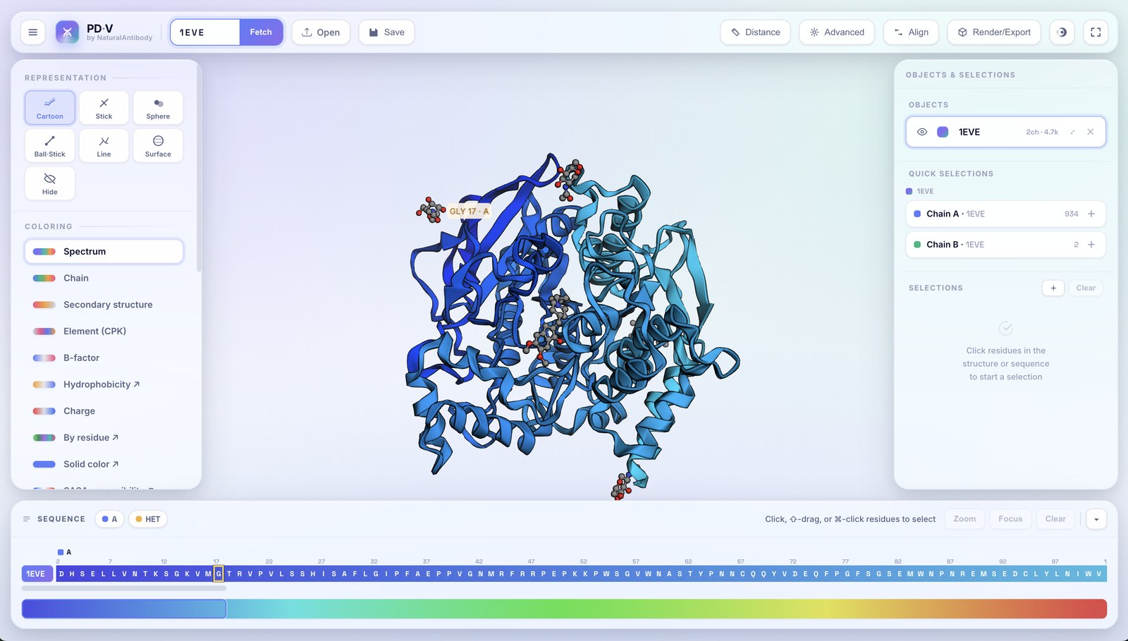
Once a structure is on screen, the whole studio comes down to six regions. Step through them below, the highlight follows along.
3Loading & objects
Every structure you load becomes an object in the right-hand Objects & Selections panel. PDV is fully multi-object.
- Additive loading: opening another file or fetching another ID adds a new object; it never replaces what's already there.
- Automatic copy naming: load the same structure twice and the second becomes
name_1, the thirdname_2, and so on. - Per-object controls: each row has an eye (show/hide), a color swatch, an editable name, a chain/atom count, zoom-to, and remove (✕).
- Active object: click an object row to target it; the left panel then edits that object.
Here's the whole loading flow, start to finish:
4Selections
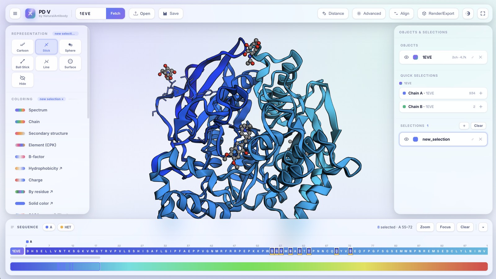
Classic named selections. The left panel (representation, coloring, style) acts on the active selection if there is one, otherwise on the active object.
- Pick residues: click residues in the 3D view or the sequence track. ⇧-drag for a range, ⌘/Ctrl-click to toggle individual residues.
- Named selections: each selection has its own color, representation, and style, layered on top of the object. Rename, recolor, hide, zoom, or delete from the panel.
- Quick selections: every chain of every object is listed (grouped under its object) as a one-click "add chain as a new selection" button.
- Editing scope: while a selection is active a small
name ×badge appears on the Representation/Coloring/Style headers; click the × to switch back to the whole object.
The right-hand panel stacks three sections, and Focus brings a pick to the foreground:
5Representations
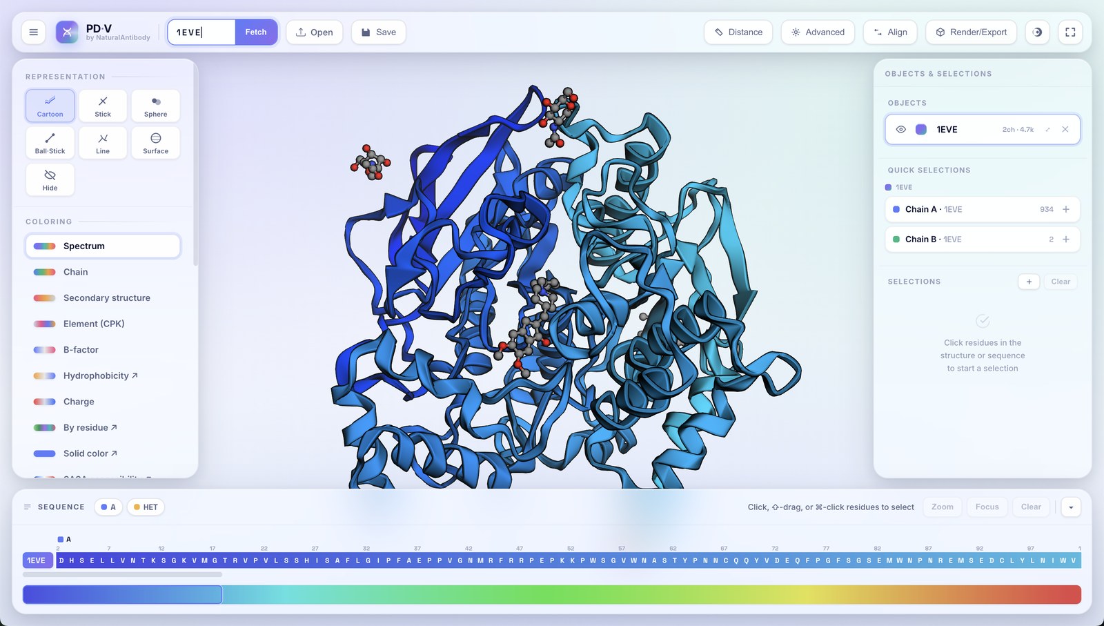
Seven representations, set per object or per selection from the Representation grid.
- Overlays preserve the base: applying a representation to a selection draws it on top of the object's representation rather than replacing it.
- Hide: removes the selected residues from view (so you can carve regions out of a surface or cartoon).
- Surface respects every coloring scheme, including per-residue ones.
Step through the seven, each on the same structure:
6Coloring
A full palette of coloring schemes, each applied to the active object or selection and mirrored onto the sequence track.
| Scheme | What it shows |
|---|---|
| Spectrum | Rainbow along the residue chain (N→C), works in every representation. |
| Chain | One color per chain. |
| Secondary structure | Helix / sheet / loop. |
| Element (CPK) | By atom element. |
| B-factor | Blue→white→red over the temperature factor. |
| Hydrophobicity | Kyte–Doolittle scale per residue. |
| Charge | Positive (blue) / negative (red) / neutral. |
| By residue… | Residue-type categories, or MSA palettes (Clustal, Zappo, Taylor), or a custom per-residue editor. |
| Solid color… | A single chosen color via the picker. |
| SASA accessibility | Solvent exposure (see Surface accessibility). |
Clicking Solid color…, By residue…, or an object/selection color swatch opens a floating color picker with a curated palette plus a custom color input. Hydrophobicity can use any of several published scales, selectable from Advanced tools → Hydrophobicity scales.
7Style controls
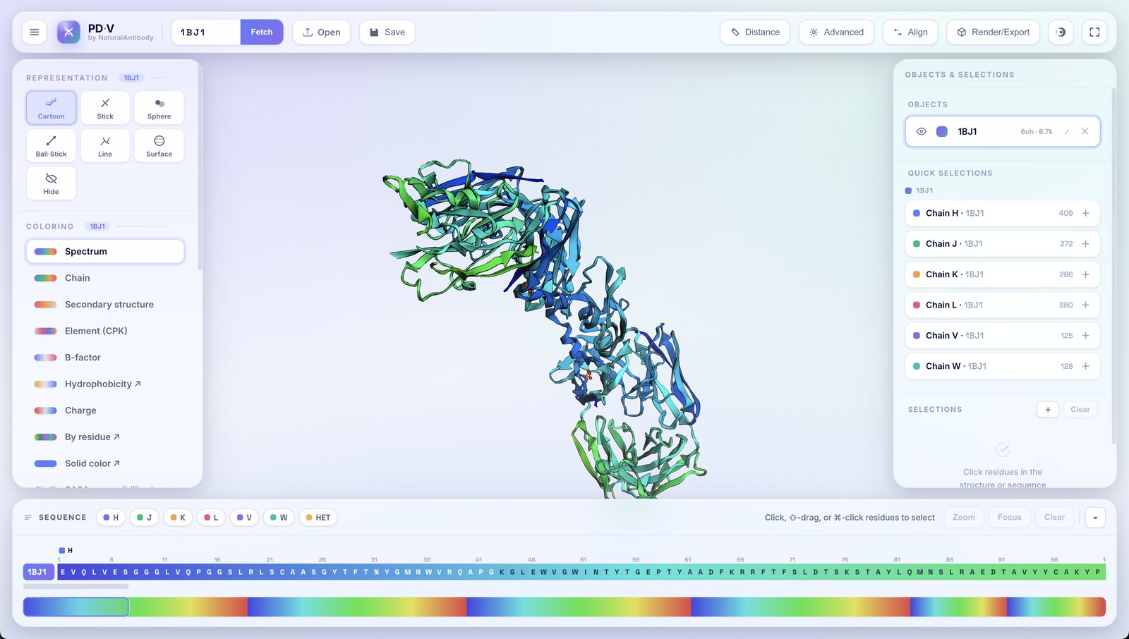
Fine-tune geometry and display. Like representation and coloring, these target the active selection if one is active, otherwise the active object.
- Sliders: cartoon thickness, stick radius, sphere size, surface opacity, and label size.
- Hydrogens: show or hide hydrogen atoms (rendered visibly even over cartoon).
- Residue labels: clean, frosted labels that scale with the label-size slider and high-resolution export.
- Spin and Depth fog: scene-wide display toggles.
8Sequence viewer
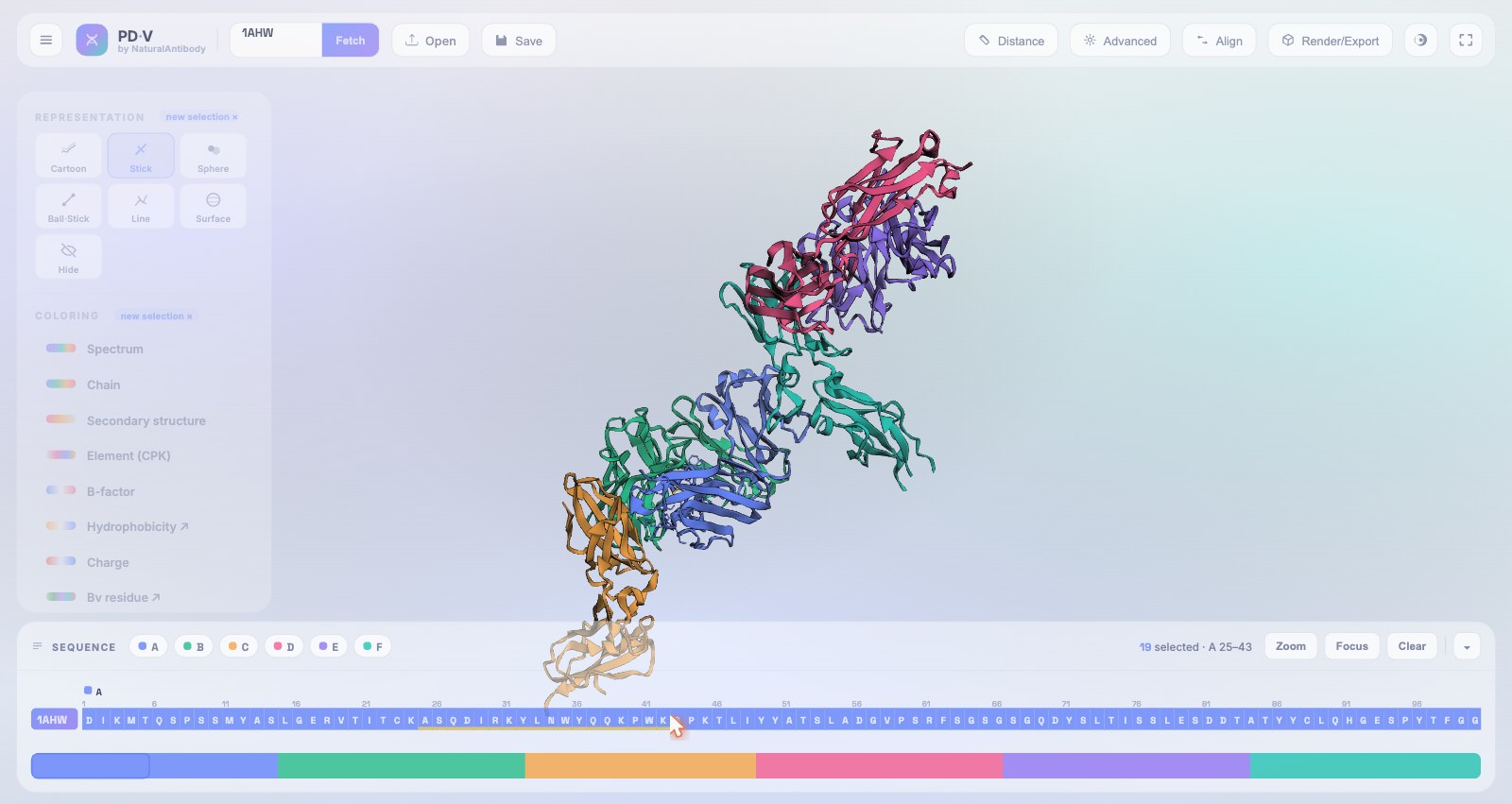
A continuous sequence track docked at the bottom, fully linked to the 3D scene.
- One continuous ribbon: all objects and chains laid out left-to-right, each prefixed by its object name and chain badge.
- Mirrors the coloring: every cell carries the same color scheme as the structure, including SASA.
- Minimap: a full-width overview with selection bands and a draggable viewport indicator.
- Navigation: chain chips (tagged by object when several are loaded) jump the track to that chain or structure.
- Two-way linking: hover a residue to highlight it in 3D and vice-versa; click to select; chain badges add a whole chain to the active selection.
docs_assets/sequence.jpg9Backdrops & view
- Backdrops: six cinematic presets (Aurora, Daylight, Mint mist, Blush, Twilight, Carbon) plus a custom-color chip. The backdrop is baked into exports.
- Full screen: the expand button (top-right) toggles full-screen mode.
- Panel toggles: collapse the left controls or right inspector to maximize the canvas; show/hide the sequence track.
10Measuring distance
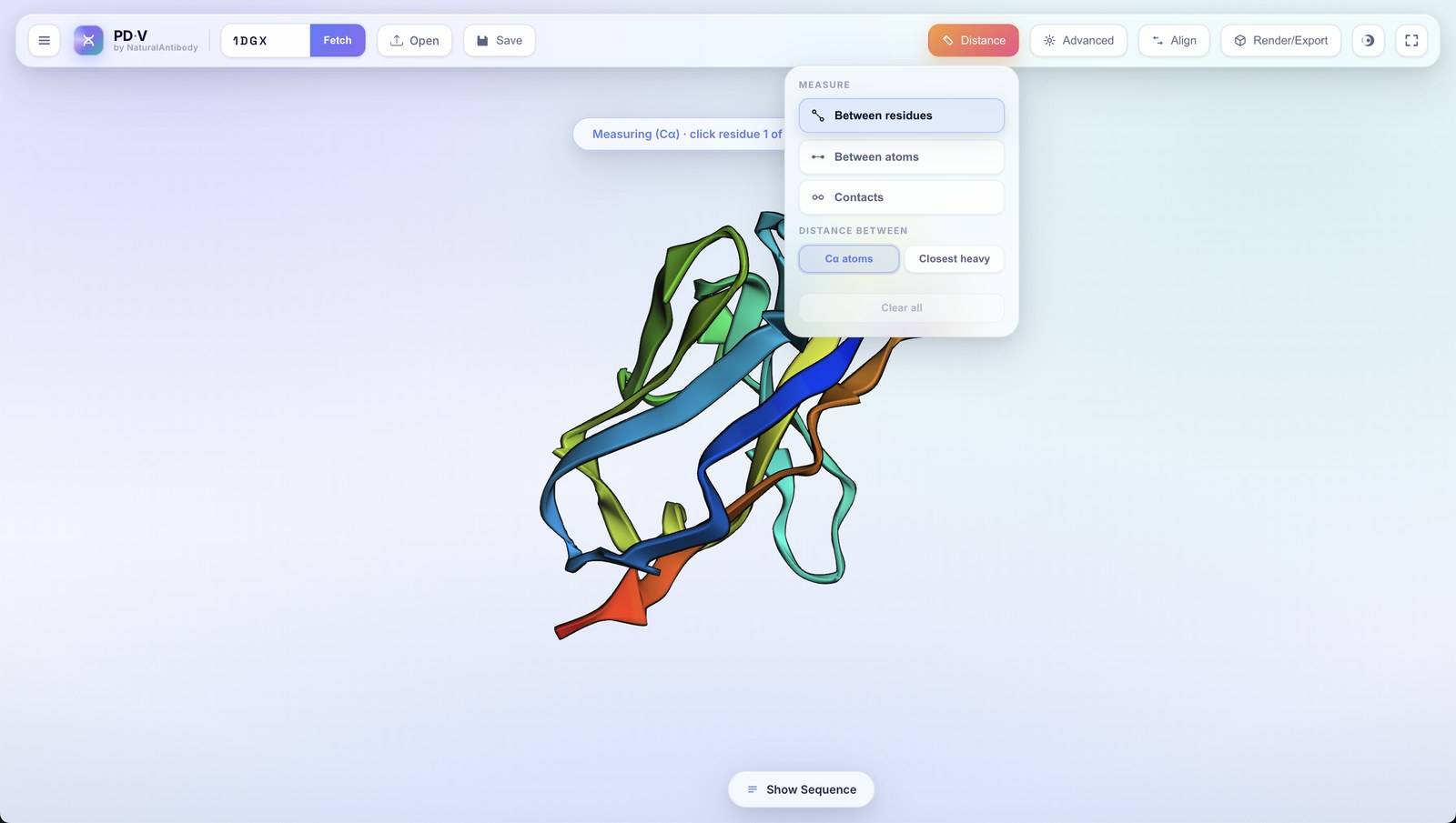
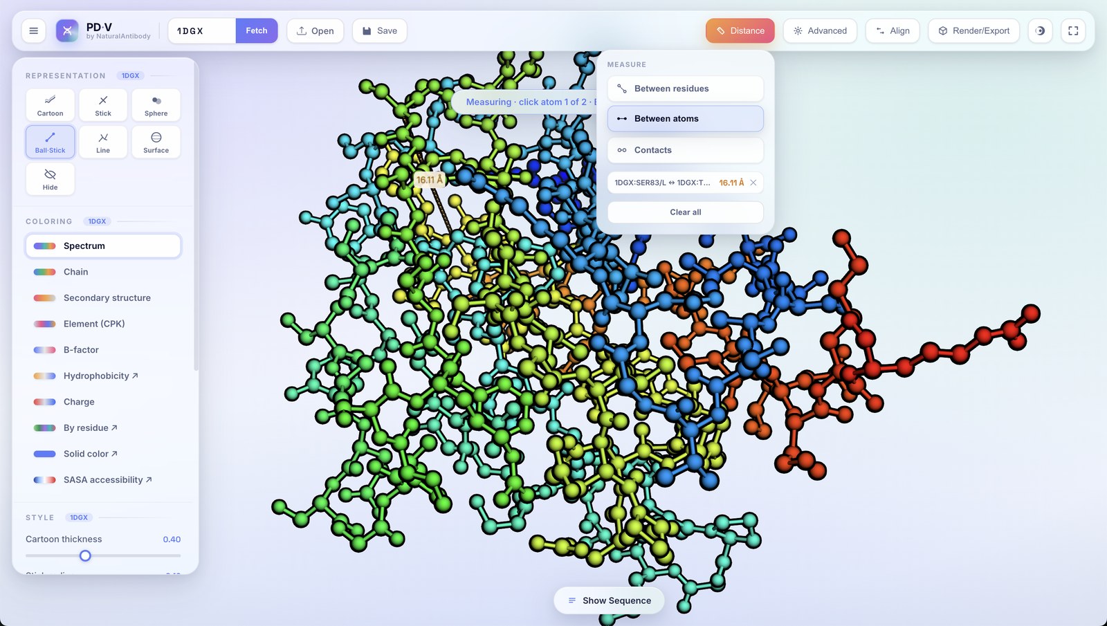
The Distance button (top bar) opens the measurement wizard.
- Between residues: pick two residues; measure either Cα–Cα or the closest heavy-atom pair (PDV finds it for you). Residues can be picked in 3D or the sequence.
- Between atoms: pick two individual atoms in 3D; pick targets tighten so you hit exactly the atom under the cursor.
Each measurement draws an orange dashed connector with endpoint halos and an Ångström label, and is listed in the panel where you can remove them individually or clear all.
Residue–residue distance
Atom–atom distance
11Contacts & non-covalent interactions
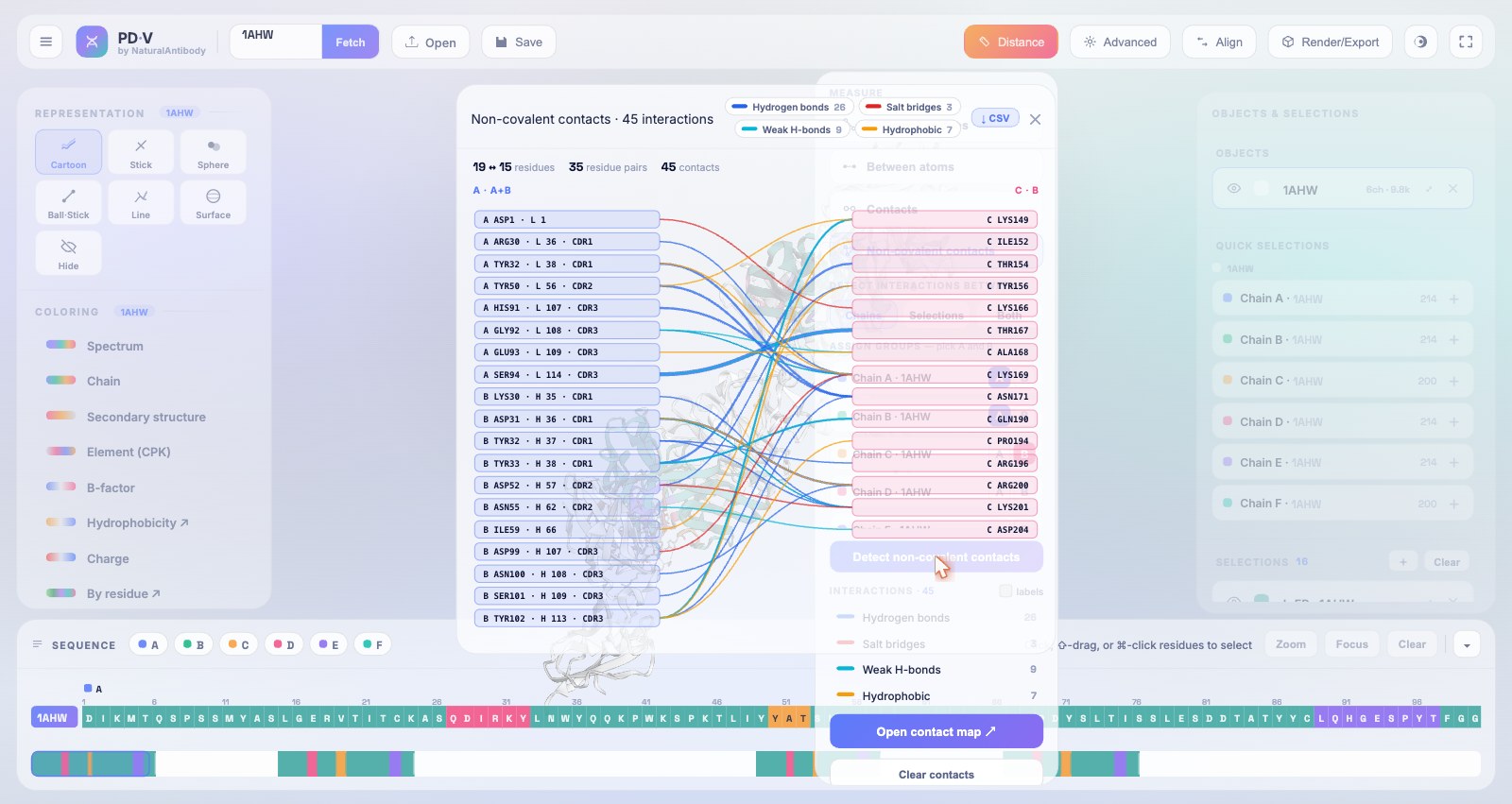
The Distance menu offers two distinct tools for mapping how two parts of a structure touch. They are easy to confuse, so the difference matters: Contacts is a pure distance search, while Non-covalent contacts classifies each contact by physical interaction type. Both run between any two groups of chains or selections.
Contacts, by distance
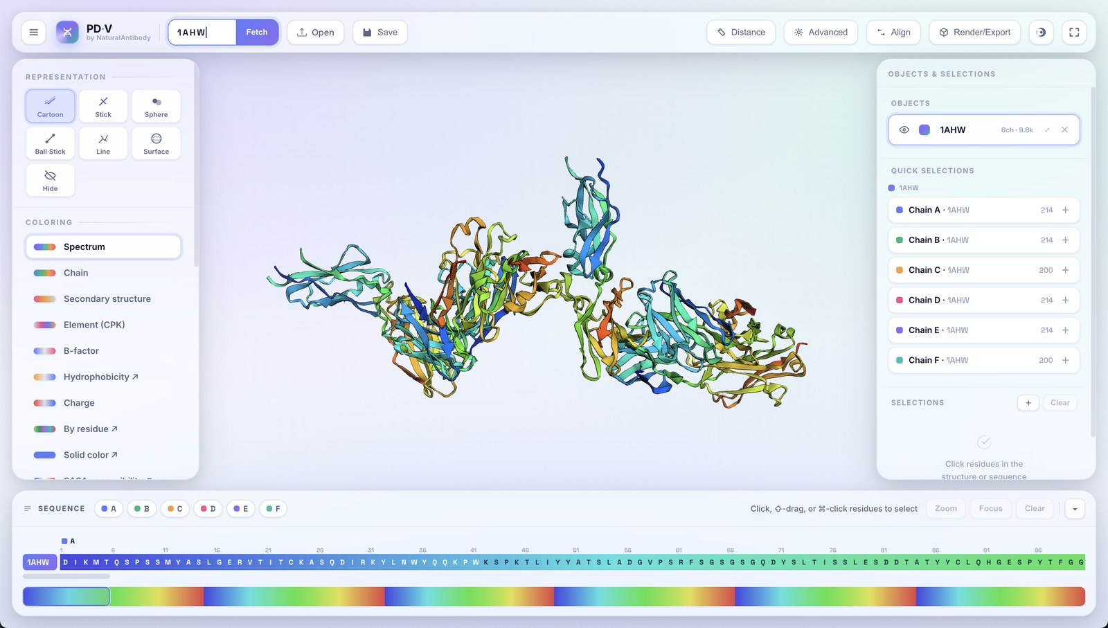
The simpler tool: a purely geometric proximity search, with no chemistry or interaction typing. Pick two groups, a distance basis and a cut-off, and PDV lists every residue pair within that distance, labelled with its actual separation. Use it when you just want "what is near what."
- Assign groups: define Group A and Group B (chains or selections).
- Distance basis & threshold: the closest heavy-atom pair or Cα–Cα, within a chosen cut-off (default 5 Å).
- Contact map: a Sankey linking the interacting residues across the two groups, labelled with each pair's distance; the residues are saved as
Contacts A/Contacts Bselections and exported to CSV.
Non-covalent contacts, by interaction type
The richer tool. Rather than a single distance cut-off, each contact is classified into a physical interaction type using PLIP-style geometric rules, and the contact map is colored by type rather than distance. Use it when you care how two residues interact, not just that they are close.
- Interaction types (van der Waals, hydrogen bonds, salt bridges, hydrophobic contacts, weak C–H···O hydrogen bonds, halogen bonds, metal coordination, water bridges, and disulfides) each from its own geometric rule (Salentin et al., 2015).
- Typed contact map: the same group-A / group-B Sankey, but grouping residue pairs by interaction category instead of distance.
docs_assets/contacts.jpg12Structural alignment
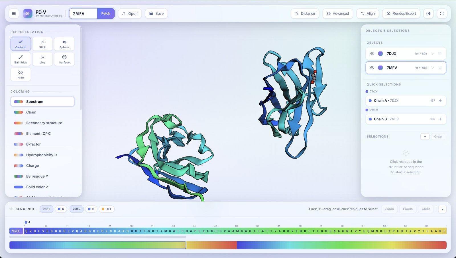
The Structural alignment button superposes one loaded object onto another so you can compare conformations or models.
- Align using: a structural superposition (Kabsch quaternion least-squares) or a sequence alignment to define the correspondence.
- RMSD: the root-mean-square deviation of the fit is reported.
13Surface accessibility (SASA)
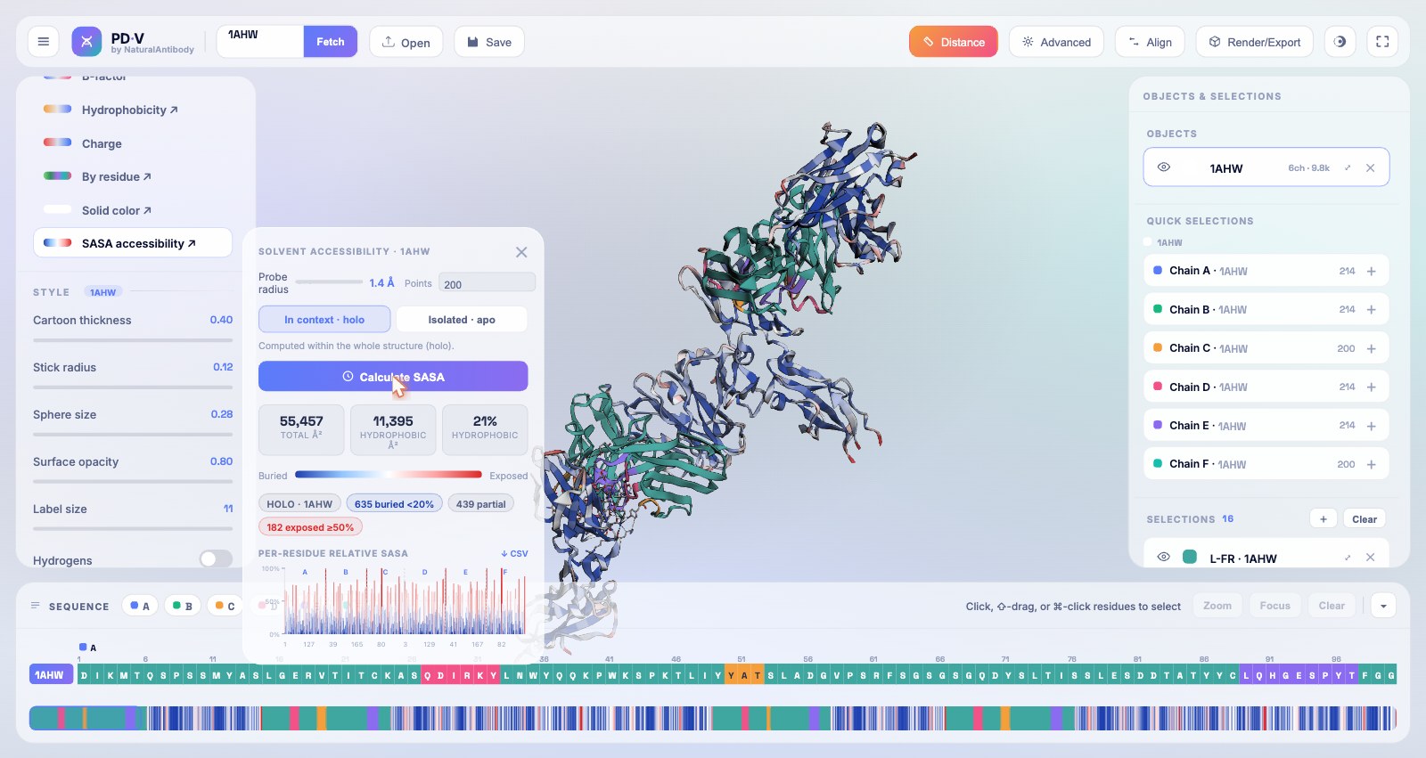
A built-in Shrake–Rupley solvent-accessible surface area engine, running in a Web Worker so the UI stays smooth.
- Pick "SASA accessibility" in the Coloring palette to open the SASA panel.
- Controls: probe radius and sampling density (points), plus a holo / apo context toggle.
- Holo computes accessibility within the whole structure; apo computes the active selection in isolation, the difference reveals the binding interface.
- Readouts: total/hydrophobic area, buried/partial/exposed counts, a per-residue bar chart, and a one-click CSV export. The structure and sequence color blue→white→red by relative exposure.
docs_assets/sasa.jpg14Antibody numbering
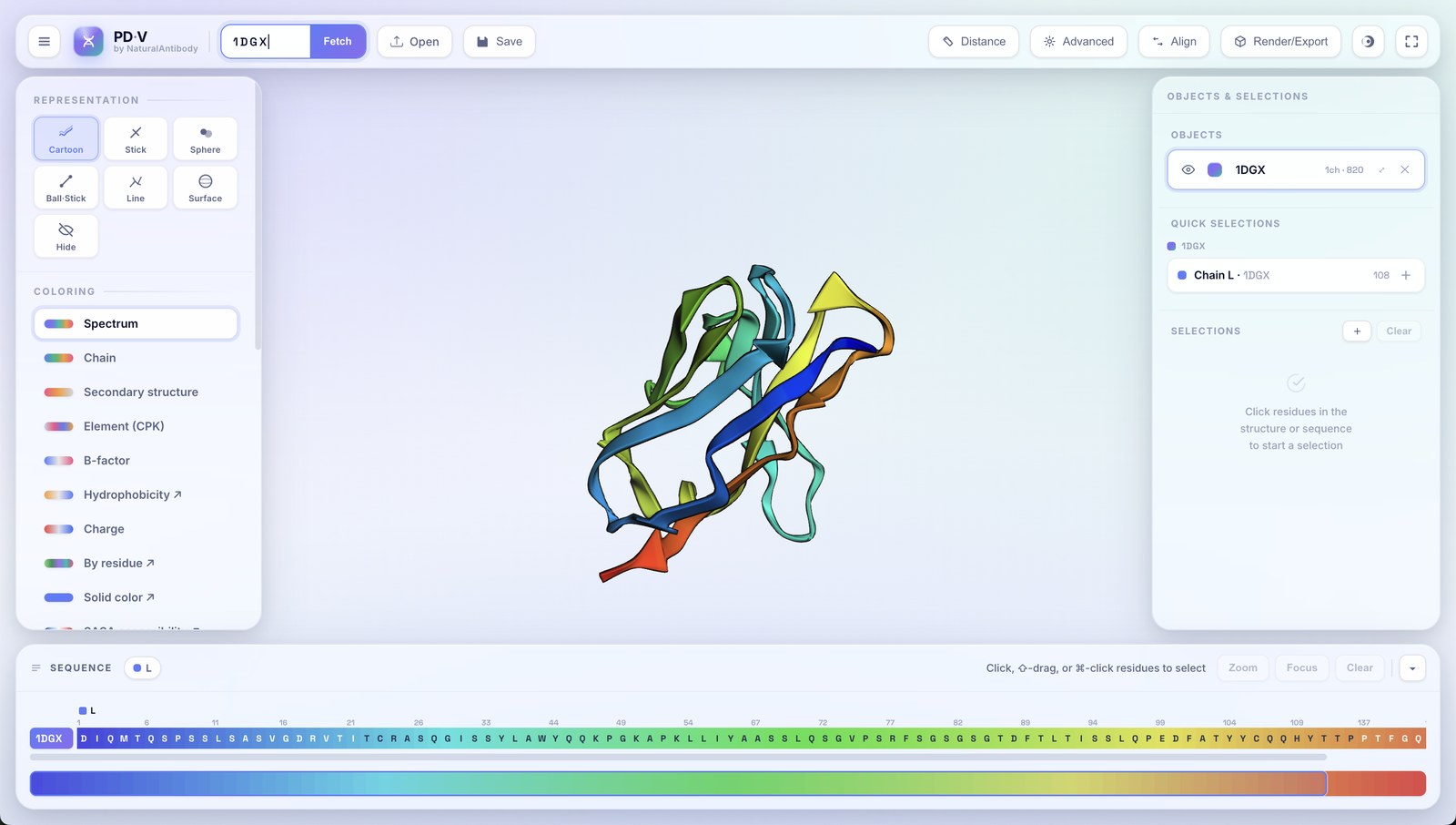
From Advanced tools → Numbering, PDV runs NaturalAntibody's RIOT engine to recognise antibody chains, apply a numbering scheme, delineate the CDRs, and assign germline genes, entirely in the browser.
- Schemes: IMGT, Kabat, Chothia, Martin (enhanced Chothia / AbM), and aHo.
- CDR delineation: CDR-H1/H2/H3 and CDR-L1/L2/L3 are detected per scheme; non-antibody chains are flagged as not an antibody.
- Germline assignment: the closest germline V (and J) genes are chosen by best local alignment.
- Two sequence views: numbered (scheme residue numbers, with insertion codes) and annotated (coloured by region: CDR, germline-identical, buried, outside-CDR).
- Report: a modal summarises the scheme, CDRs, and germline calls per chain.
15Developability liabilities
Advanced tools → Liabilities scans for common antibody developability motifs and ranks them by how genuinely risky they are in this structure.
- Motifs detected: Asn deamidation, Asp isomerization, N-glycosylation sequons, Met and Trp oxidation, metal-catalysed His oxidation, fragmentation / cleavage sites, and unpaired / missing cysteines.
- Context-weighted: each hit is scored by structural context: solvent exposure, proximity to the CDRs, and whether it is germline-encoded. An exposed, CDR-proximal, non-germline motif is flagged as genuinely risky; a buried or germline one is down-weighted.
- Linked highlighting: liabilities are marked on both the structure and the sequence track.
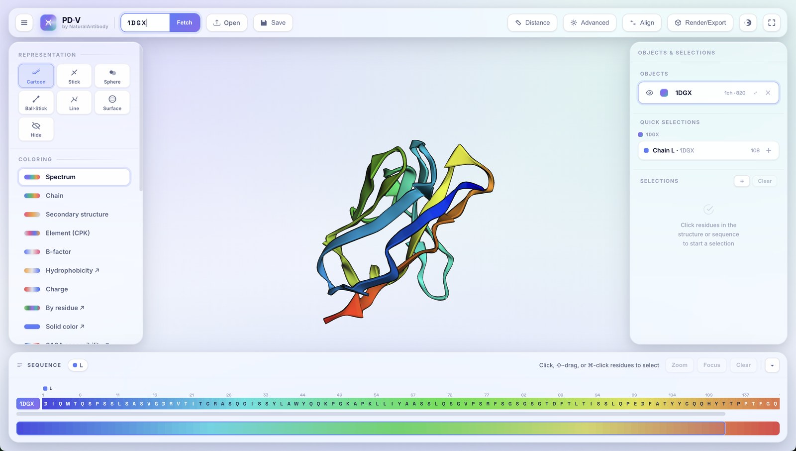
16Disulfide bonds
Advanced tools → Disulfide bonds finds every cystine bridge in the loaded structures and draws it straight onto the molecule, even in cartoon views, where the underlying renderer never draws covalent bonds at all.
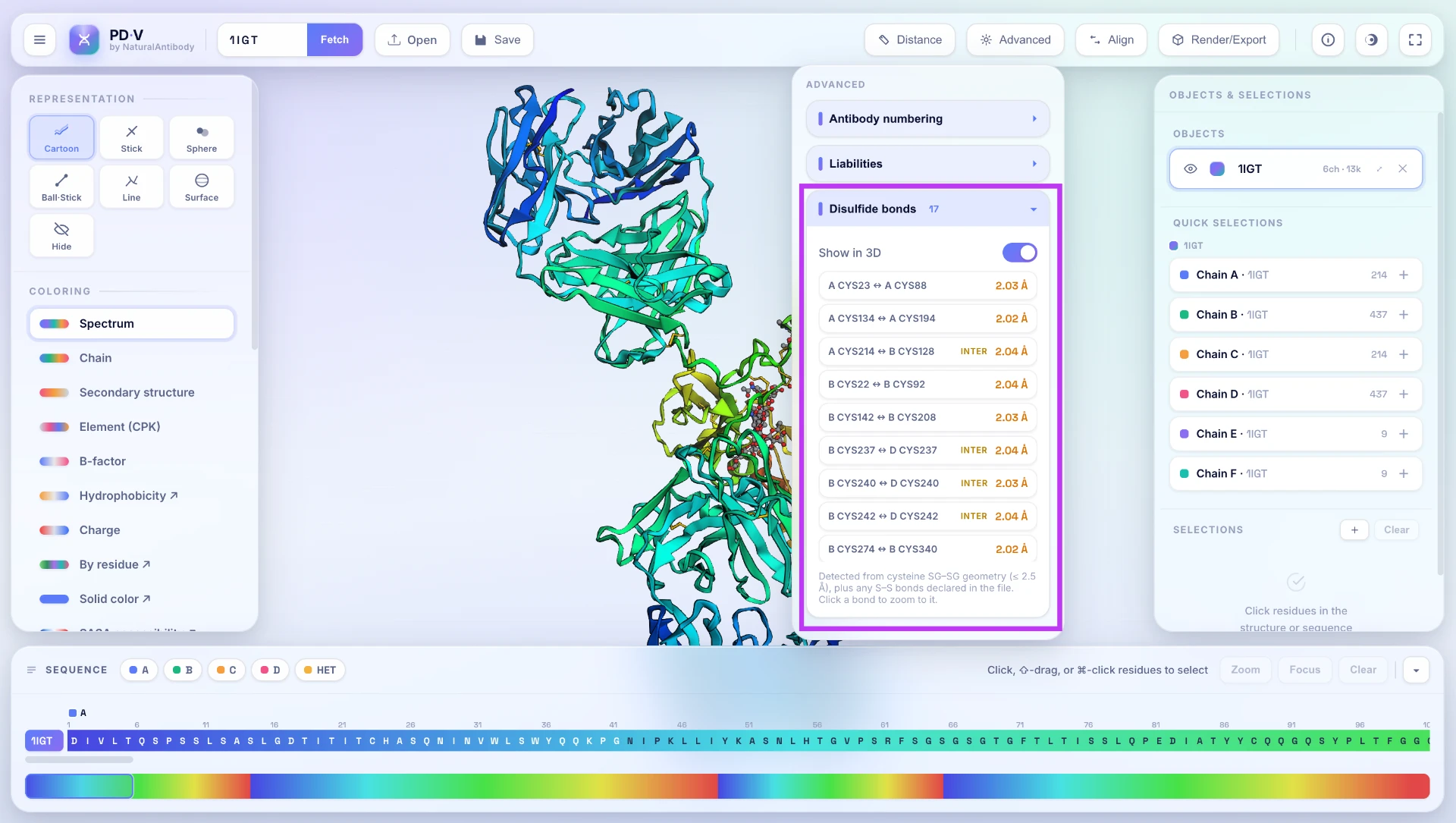
disulfide.webp- How bonds are found: PDV measures the distance between the γ-sulfur atoms (SG) of every pair of cysteines and keeps pairs within 2.5 Å. An ideal S–S bond is ≈ 2.04 Å, so the cutoff tolerates modelled or lower-resolution coordinates. S–S bonds explicitly declared in the file (PDB
CONECTrecords) are also kept, up to 3.0 Å. - Drawn on top of any representation: each bridge is rendered as a bright yellow overlay, with cylinders along the
CA → CB → SGside-chain path of both cysteines, theSG–SGbond itself, and small spheres marking the two sulfur atoms. Because it is an overlay, disulfides stay visible in every representation. In stick or line views, detected bonds are also added to the model's bond list, so hover highlighting and selection treat them as ordinary bonds. - The bond list: every bond is listed in the section, labelled
chain · residue ↔ chain · residuewith its measured S–S distance in Å. Bridges spanning two chains carry an inter tag; hovering a row shows whether the bond was declared in the file or detected by geometry. When antibody numbering has been applied, rows also carry the numbered residue label. With several structures loaded, the list is grouped per object with a per-object count, and the badge on the section header totals all bridges. - Click to zoom: clicking a bond in the list zooms the camera to that bridge, framing both cysteines.
- Works with selections: with a selection active, bonds involving the selected residues stay at full strength while all others fade to 15%, so you can select the CDRs, for example, and still see which disulfides pin them down.
17Rendering & export
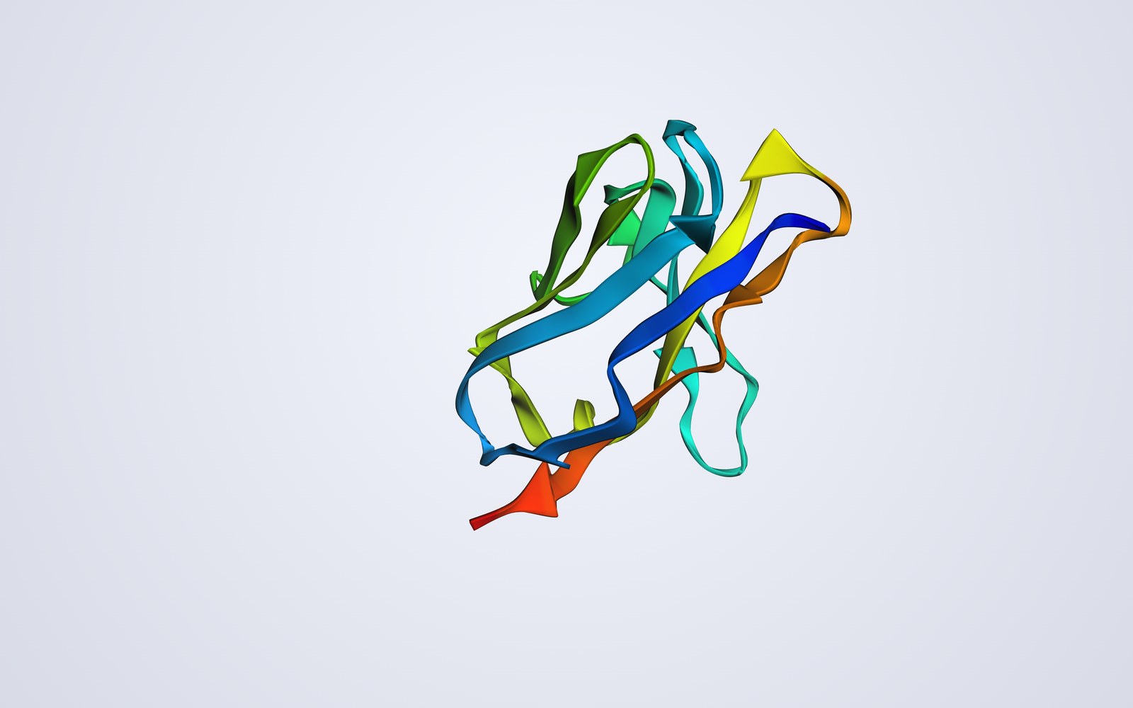
The Render/Export button produces publication-quality PNGs with several render modes.
| Mode | Look |
|---|---|
| No outline | Plain shaded render. |
| Outline · default | Clean dark contour around the molecule. |
| Cartoon | Bold thick ink outline. |
| Line art | Outline-only line drawing on a white background. |
| Cel shade | Quantized colors + outline (mode 3). |
- Outline color: sets the contour color; pick black, ink, magenta, blue, teal, or a custom color.
- Output quality: 1×, 2×, or 4× supersampling (auto-capped to your GPU's limit); labels scale so they stay readable.
The same view (1DGX), exported in each mode:
18Sessions
The Save session button writes the entire scene to a portable .mvsession file.
- What's saved: every loaded object, its representation, coloring and style, all named selections, and the camera view.
- Portable: reopen the session later to restore the scene exactly, or hand the file to a colleague alongside the single-file app.
19Keyboard shortcuts
Available when the cursor isn't in a text field.
| Key | Action |
|---|---|
| C | Cartoon representation |
| S | Stick representation |
| B | Sphere representation |
| L | Line representation |
| F | Surface representation |
| R | Reset / recenter the view |
| M | Open the Distance (measure) wizard |
| Esc | Stop measuring · close popovers |
Mouse: drag to rotate, scroll to zoom, right-drag (or two-finger) to pan, double-click a residue to zoom to it, right-click an atom for the context menu.
20Privacy & offline
PDV is a single HTML file. Apart from optionally fetching a structure from the RCSB when you type a PDB ID, nothing leaves your computer, files you open are parsed and rendered locally in WebGL. Save the file anywhere and it keeps working with no internet connection.
21Licensing
PDV is free for noncommercial use under the PolyForm Noncommercial License 1.0.0. Commercial use requires a one-time license: between USD 100-500, per organization (depending on organization size), perpetual. © 2026 NaturalAntibody.
Free for noncommercial use
Academics, students, nonprofits, and hobbyists can download and use PDV at no cost under the PolyForm Noncommercial License 1.0.0.
Commercial license: USD 100-500 per organization, perpetual
Using PDV in a company or for commercial work? A one-time fee between USD 100-500 covers your whole organization, forever. Get in touch to purchase.
How to buy
- Download PDV and try it free.
- If your organization uses it commercially, contact us at naturalantibody.com/contact-us to purchase the perpetual license (USD 100-500 per organization).
- We send the license confirmation for your organization.
FAQ
Is PDV really free? Yes, for noncommercial use (research, teaching, personal, nonprofits) under the PolyForm Noncommercial License 1.0.0.
When do I need to pay? If you or your organization use PDV for commercial purposes. The fee is between USD 100-500 per organization (depending on organization size), perpetual.
What does “per organization, perpetual” mean? One payment covers your whole organization (and entities it controls), with no expiry, for PDV.
How do I pay? Contact us at naturalantibody.com/contact-us and we’ll handle it. There is no self-serve checkout.
What open-source software does PDV use? PDV is built on 3Dmol.js (BSD-3-Clause) and other open-source libraries (GLmol, Three.js, jQuery, pako, and an FXAA shader, MIT), plus germline reference data from OGRDB (public domain / CC0). Full notices ship inside the app and are listed below.
Open-source attributions
Ready to visualize?
Open the studio in a new tab and load your first structure.